Our product is meant to work on whatever model an engineer already uses. That makes model choice a question we have to answer repeatedly, for customers and for our own defaults, and since the spring the honest answer has been that we cannot tell most of the candidates apart. The published evidence is almost always a single number on a small benchmark, reported without an interval, compared with another single number from a different run with a different sampling temperature.
This paper asks how much of the difference between two such numbers is signal. It is a simulation study, because the question is about the measurement procedure rather than about any particular model, and because in a simulation the true difference is known. We are not ranking real models here and we make no claim about any of them.
What a benchmark score is an estimate of
A code benchmark is a sample of m problems, each with a hidden test suite. For a given model and decoding setting, problem j has a true probability pj that a sampled completion passes. Drawing n completions and counting cj passes, the benchmark reports
where the second expression is the unbiased estimator introduced with HumanEval by Chen and colleagues. Two different quantities are being estimated, and leaderboards rarely say which. The benchmark estimand is the mean of pj over these particular problems; its uncertainty comes only from sampling completions. The capability estimand is the mean over the population of problems the benchmark stands for; its uncertainty also includes which problems happened to be chosen. Anyone using a leaderboard to choose a model for their own code wants the second.
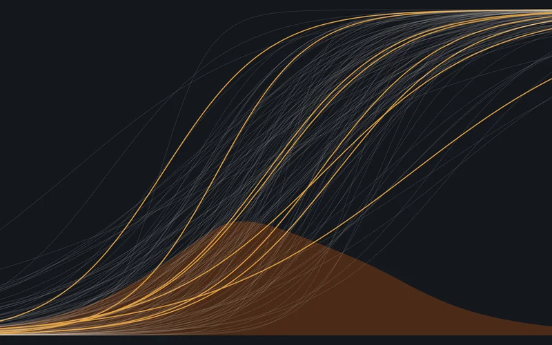
Our generator gives each problem a latent difficulty dj ~ N(0, 1.9²), which reproduces the familiar shape of code benchmarks: a block of problems nearly every model solves, a block nearly none do, and a contested middle. A model with skill s solves problem j with probability expit(s − dj + εj), where εj ~ N(0, 0.6²) is a model-specific affinity for that problem, so two models agree on which problems are hard but not perfectly. Skill is solved numerically so that the model’s true pass@1 hits a target, usually 45%.
Result 1: the naive pass@k is biased, the published one is not
A common shortcut computes pass@k as 1 − (1 − c/n)k, plugging the per-problem pass rate into the formula for k independent tries. By Jensen’s inequality this is biased downward whenever n is small relative to k.
At n = k = 10 the plug-in understates pass@10 by 5.0 points (83.1% against a true 88.2%); at n = 20 it is still 2.3 points low, and only at n = 200 does the bias fall to a quarter of a point. The unbiased estimator in (1) was within a quarter of a point of the truth in every configuration, a residual consistent with Monte Carlo noise. This is a solved problem, and we include it only because the shortcut still appears in evaluation scripts. Its effect is to penalise whichever model was sampled fewer times.
Result 2: most of the noise is in the problems, not the samples
The more consequential issue is variance. We decompose the standard deviation of the benchmark score into the part due to sampling completions (holding the problem set fixed) and the total (also redrawing the problems from the same population).
With one sample per problem on 164 problems, the score has a standard deviation of 3.9 points, of which completion sampling contributes most. Drawing ten samples per problem removes that component almost entirely, but the total only falls to 2.7 points, because 88% of what remains is problem sampling, which no amount of resampling the model can reduce. At 100 samples per problem, 98% of the variance comes from which 164 problems were chosen. The same pattern holds at 500 problems (2.3 points total at one sample, 1.5 at ten) and at 2,294 (1.0 and 0.7).
A leaderboard reports a number whose uncertainty is dominated by a source that its usual error bar, when it has one at all, leaves out. More samples tighten the interval around ‘how this model does on these 164 problems’. They do almost nothing for ‘how this model will do on yours’.
Result 3: compare models on the same problems, and say so
When two models are evaluated on the same problems, the problem-sampling variance is largely shared and cancels in the difference, provided the test uses the pairing. The paired estimate and its standard error are
which for n = 1 reduces to McNemar’s test on the discordant problems. The alternative found in most comparisons treats each model’s m·n completions as independent Bernoulli trials and runs a two-proportion test. We measured both when the two models are in fact equally good.
| Benchmark | Samples per problem | Unpaired binomial test | Paired test over problems |
|---|---|---|---|
| 164 problems | 1 | 1.7% | 5.5% |
| 164 problems | 5 | 3.2% | 5.2% |
| 164 problems | 20 | 10.7% | 5.5% |
| 500 problems | 1 | 2.0% | 4.7% |
| 500 problems | 5 | 3.2% | 5.7% |
| 500 problems | 20 | 9.8% | 5.2% |
The unpaired test is wrong in both directions. At one sample per problem it ignores the correlation between the models and is too cautious, rejecting 1.7% of the time when it claims 5%. At twenty samples it treats repeated completions of the same problem as independent evidence and becomes too eager, declaring a difference in one comparison in ten when there is none. The paired test holds its nominal rate everywhere.
Correct calibration does not buy much power on a small benchmark. For a true three-point gap on 164 problems, the paired test detects it 7% of the time with one sample per problem and 51% with twenty. On 500 problems the figures are 16% and 93%; on 2,294, 72% and 100%. Inverting the calculation gives the minimum detectable effect at 80% power:
| Benchmark | One sample per problem | Ten samples per problem |
|---|---|---|
| 164 problems (HumanEval) | 12.4 points | 4.9 points |
| 500 problems (MBPP test) | 7.1 points | 2.8 points |
| 2,294 problems (SWE-bench) | 3.3 points | 1.3 points |
A greedy-decoding comparison on HumanEval cannot reliably detect anything smaller than about twelve points. Most of the gaps that separate adjacent entries on this year’s leaderboards are a fraction of that.
Result 4: rankings flip
Leaderboards are read as orderings. We simulated five models with true pass@1 of 40%, 41.5%, 43%, 45% and 47%, a spread typical of the dense middle of a leaderboard, and evaluated each once with a single sample per problem.
On 164 problems the full order is right 9% of the time and the best model is on top 63% of the time. On 2,294 problems those become 71% and 94%. A practitioner choosing among the middle of a HumanEval leaderboard is very largely choosing at random, and should expect a different ordering from anyone else who reruns it.
Result 5: a little contamination outweighs a lot of signal
Benchmarks published before a model’s training cut-off may be in its training data. We modelled contamination crudely: a share of problems the model has memorised and solves 97% of the time regardless of difficulty.
Memorising 5% of HumanEval adds 3.1 points; 10% adds 5.6; 20% adds 10.7. Because the memorised problems are concentrated among those the model would otherwise fail, the inflation is larger than the share contaminated. A model that has seen one problem in ten gains more than the typical gap between adjacent leaderboard entries, and nothing in the reported number distinguishes that from capability. Held-out and freshly written problem sets, of the kind EvalPlus and SWE-bench move toward, are the only defence.
Result 6: tasks from the same repository are not independent
Repository-level benchmarks such as SWE-bench draw many tasks from each repository, and tasks from the same codebase share difficulty. That correlation inflates variance by the design effect familiar from survey sampling, 1 + (b − 1)ρ for clusters of size b and intra-cluster correlation ρ.
| Structure (2,294 tasks) | SD of pass@1 (points) |
|---|---|
| Independent tasks | 1.06 |
| 5 tasks per repository, ρ = 0.2 | 1.16 |
| 12 tasks per repository, ρ = 0.2 | 1.44 |
| 12 tasks per repository, ρ = 0.4 | 1.74 |
Because ρ here is defined on the latent difficulty scale, the correlation of pass/fail outcomes is smaller and the observed variance inflation (1.9 and 2.7 for the last two rows) is below what the formula gives with latent ρ. Even so, with twelve tasks per repository a 2,294-task benchmark has the precision of roughly 1,240 independent tasks at ρ = 0.2 and 850 at ρ = 0.4. The appropriate interval resamples repositories, not tasks. SWE-bench draws from a small number of repositories, so this correction is not a technicality there.
What we recommend
- Report pass@1 with a paired interval against a named baseline evaluated on the same problems, using (2), or McNemar’s test at one sample.
- Use the unbiased pass@k estimator, and never compare pass@k values computed from different numbers of samples.
- Sample at least ten completions per problem when the decoding is stochastic, and report the temperature.
- Resample at the repository level for repository-sourced benchmarks.
- Treat any gap smaller than the detectable effect in the table above as a tie, and decide on other grounds (latency, cost, licence, whether the model runs locally).
- Evaluate on your own held-out tasks for the decisions that matter, because public benchmarks answer a different question and may be contaminated.
Method
Limitations
The generator is a one-dimensional difficulty model with independent model-specific noise. Real models differ in kind as well as degree, solving different families of problem, which would make pairing less effective than it is here and our power figures optimistic. Pass rates also depend on the test suites, which for HumanEval are known to be thin; a model can pass a weak suite with incorrect code, which adds a bias our simulation does not contain. Our contamination model is the crudest possible. Finally, none of this says whether a benchmark measures what an engineer needs from a model in a real codebase, which is a question only evaluation on one’s own code can answer.
Simulation only. No real model was evaluated for this paper and none is named in the results. Scripts and seeds are published under Artefacts.
Related work
The unbiased pass@k estimator and HumanEval come from Chen and colleagues [1]; MBPP from Austin and colleagues [2]; SWE-bench from Jimenez and colleagues [3]. Liu and colleagues [4] showed that HumanEval’s tests are thin enough to change rankings once strengthened, a measurement problem complementary to the sampling problem studied here. On significance testing for model comparisons, Dror and colleagues [5] survey the options and Card and colleagues [6] show how often NLP comparisons are underpowered; our minimum detectable effects are the code-generation analogue. Bouthillier and colleagues [7] decompose benchmark variance into sources in a way that parallels our problem and sample components. McNemar [8] gives the paired test at one sample, Kish [9] the design effect, and Efron and Tibshirani [10] the bootstrap we recommend at repository level. Sainz and colleagues [11] set out the contamination problem for language-model benchmarks. The comprehension instrument we use for our own evaluations is described in AWL-2023-01 [12].
Artefacts
Everything below is published or available on request. A number nobody can reproduce is an advertisement, not a result.
References
- Chen, M., Tworek, J., Jun, H., et al. (2021). Evaluating Large Language Models Trained on Code. arXiv:2107.03374.
- Austin, J., Odena, A., Nye, M., et al. (2021). Program Synthesis with Large Language Models. arXiv:2108.07732.
- Jimenez, C. E., Yang, J., Wettig, A., Yao, S., Pei, K., Press, O., & Narasimhan, K. (2023). SWE-bench: Can Language Models Resolve Real-World GitHub Issues? arXiv:2310.06770.
- Liu, J., Xia, C. S., Wang, Y., & Zhang, L. (2023). Is Your Code Generated by ChatGPT Really Correct? Rigorous Evaluation of Large Language Models for Code Generation. arXiv:2305.01210.
- Dror, R., Baumer, G., Shlomov, S., & Reichart, R. (2018). The Hitchhiker’s Guide to Testing Statistical Significance in Natural Language Processing. ACL.
- Card, D., Henderson, P., Khandelwal, U., Jia, R., Mahowald, K., & Jurafsky, D. (2020). With Little Power Comes Great Responsibility. EMNLP.
- Bouthillier, X., Delaunay, P., Bronzi, M., et al. (2021). Accounting for Variance in Machine Learning Benchmarks. MLSys.
- McNemar, Q. (1947). Note on the Sampling Error of the Difference Between Correlated Proportions or Percentages. Psychometrika, 12(2).
- Kish, L. (1965). Survey Sampling. Wiley.
- Efron, B., & Tibshirani, R. J. (1993). An Introduction to the Bootstrap. Chapman and Hall.
- Sainz, O., Campos, J. A., García-Ferrero, I., Etxaniz, J., Lopez de Lacalle, O., & Agirre, E. (2023). NLP Evaluation in Trouble: On the Need to Measure LLM Data Contamination for Each Benchmark. Findings of EMNLP.
- Bhardwaj, M. (2023). An item bank for code comprehension: calibration, adaptive testing and fairness checks with item response theory. AI Work Lab Research, AWL-2023-01.
Bhardwaj, M. (2023). Pass@k is not a ranking: the statistics of code-model leaderboards. AI Work Lab Research, AWL-2023-02.