Every AI coding assistant emits the same telemetry: a suggestion was shown, it was accepted or not, and some time passed in between. Vendors summarise it as acceptance rate, and engineering managers have started to put acceptance rate on dashboards. We think it measures the wrong thing. A suggestion accepted after six seconds of reading and then adjusted is a different act from one accepted in under a second and never looked at again, and it is the second one we worry about.
Barke, James and Polikarpova observed that programmers working with completion tools move between an acceleration mode, where they know what they want and accept quickly, and an exploration mode, where they read and weigh suggestions. Mozannar and colleagues went further and labelled programmer activity in fine-grained states from screen recordings. Both point at the same structure: what matters is a latent state that the telemetry only partly reveals. That is the definition of a hidden Markov model. This paper builds one, tests it where the truth is known, and tries to break it.
A simulation study. Every engineer, session and event is generated by the script under Artefacts, including the link between review state and comprehension used in Result 3, which is an assumption of the simulation, not a finding. What the paper tests is whether the model can recover structure that is there, and how its summaries behave under pressure.
The model
Within a coding session, engineer i sees a sequence of suggestions t = 1, ..., T. Each produces an outcome ot in {reject, accept unchanged, accept then edit} and a dwell time dt from display to decision. A latent state zt in {E, S, R} (engaged, skim, rubber-stamp) follows a first-order Markov chain, and the observations are conditionally independent given the state:
The outcome distribution θk and the dwell distribution are what give the states their meaning. Nothing in the fitting tells the model which state is ‘engaged’; we name them afterwards from their fitted emissions. That turns out to matter in Result 4.
Fitting
Parameters are estimated by the Baum-Welch algorithm, the EM algorithm for hidden Markov models, with the forward and backward recursions computed in log space and vectorised across 7,200 sessions of 20 to 70 events. The E-step computes the posterior state probabilities γt(k) and pairwise transition posteriors ξt(j, k):
and the M-step re-estimates A from expected transition counts, θ from γ-weighted outcome counts, and (μ, σ) from γ-weighted moments of log dwell. Each fit used three initialisations and kept the one with the highest likelihood. The number of states was chosen by the Bayesian information criterion, with K(K − 1) transition, K − 1 initial, 2K outcome and 2K dwell parameters.
Simulated engineers
The fatigue effect is deliberate misspecification. Real behaviour will not be a homogeneous Markov chain, and a model that only works when it is exactly right is not worth deploying.
Result 1: the structure is recoverable
| States | BIC | Difference from best |
|---|---|---|
| 2 | 1,177,529 | +40,981 |
| 3 | 1,136,548 | 0 |
| 4 | 1,136,682 | +134 |
BIC prefers three states, and by a wide margin over two. The fourth state buys a little likelihood, but not enough to pay for its parameters. The fitted emissions are close to the generating ones: dwell-time means of 6.02, 2.20 and 0.90 seconds against 6.0, 2.2 and 0.9, and the rubber-stamp state accepts unchanged 94.0% of the time against 94%.
Viterbi decoding assigns 90.8% of events to the correct state. Engaged review and rubber-stamping are almost never confused with each other (0.2% and 0.1% of events); the errors are between skim and its neighbours, which is where the states genuinely overlap. Even though the model assumes a constant transition matrix, the posterior share of rubber-stamping rises across a session from 34% in the first ten suggestions to 51% after the fiftieth, against a true 33% and 52%. The posterior is driven by the emissions, so drift in the dynamics shows up in the decoding anyway.
Result 2: better than a stopwatch
The obvious alternative is a rule: call any acceptance with a dwell under 1.5 seconds a rubber stamp. It is not bad.
| Rubber-stamp detector | Precision | Recall |
|---|---|---|
| Dwell under 1.5 s and accepted | 88.6% | 84.5% |
| HMM, Viterbi path | 93.4% | 94.9% |
The HMM gains on both, mainly because it uses context: a quick acceptance in the middle of a run of careful reviews is probably a skim of something obvious, while the same quick acceptance in a run of quick acceptances is probably not. That is the transition matrix doing its work.
Result 3: which summary tracks understanding
The reason to decode review states is to say something about engineers. We computed four engineer-level summaries and correlated each with the simulated comprehension outcome.
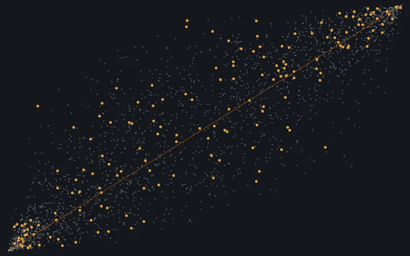
Before gaming, the three summaries built from dwell time all correlate about as well with the outcome (−0.55 to −0.56, or +0.55 for mean dwell), and acceptance rate somewhat worse (−0.48). The HMM’s advantage over the heuristic at the event level mostly averages out at the engineer level, which is an honest result and a useful one: if nobody is gaming the measure, a stopwatch is nearly as good.
Result 4: when engineers learn what is being watched
Any summary that becomes a target will be optimised. The cheapest way to look engaged on a dwell-time measure is to wait three seconds before pressing tab. We simulated exactly that: rubber-stamp dwell moves from about 0.9 to about 3.2 seconds, and nothing else about the behaviour changes.
The dwell-time rule collapses: its correlation with comprehension goes from −0.55 to +0.07, because rubber-stamp acceptances now take longer than 1.5 seconds. An HMM fitted before the change and left frozen fails the same way (+0.11), because it learned that rubber-stamping is fast. Mean dwell time weakens from +0.55 to +0.35. Acceptance rate is untouched at −0.50, since waiting does not change what is accepted, so for the moment the crudest metric on the dashboard is the best one.
Refitting the HMM on the new telemetry finds three states again. The rubber-stamp state now has a mean dwell of 3.2 seconds, but it still accepts unchanged 94% of the time and edits 3% of the time, so it is recognisable by its behaviour. Named that way, its engineer-level share correlates −0.53 with comprehension, almost all of the pre-gaming −0.56. The first version of this analysis named states by speed, labelled the skim state as rubber-stamping after the refit, and reported a correlation of +0.28; version 1.1 corrects that. The correction is the lesson: a behavioural model survives gaming only if its states are defined by what people do, not by the signal they can most easily change.
A dwell-time or acceptance-based score should not be shown to managers. The defensible use of a review-state model is narrower: deciding when to ask an engineer to explain a change, a use that does not reward gaming it, with the model refitted on a schedule rather than frozen.
Method
Limitations
The simulated engineers have exactly three review states, so finding three is reassurance about the fitting, not evidence about people; real behaviour may need more states, or a continuum. The link to comprehension is assumed, and the whole point of the cohort study we are planning is to measure it rather than assume it. Telemetry differs by tool, and some tools do not expose dwell or post-acceptance edits at all. Finally, the gaming scenario is one specific adaptation; engineers who learn to edit trivially after accepting would attack the outcome channel instead, and we have not simulated that.
Simulation only. No engineer or customer telemetry was used. Script, seed and results file are under Artefacts.
Related work
Hidden Markov models and the Baum-Welch algorithm are Baum and colleagues [1]; Rabiner [2] is the standard tutorial and Zucchini, MacDonald and Langrock [3] the reference for applied work. Model selection uses Schwarz [4] and decoding Viterbi [5]. The states we model follow the acceleration and exploration modes described by Barke, James and Polikarpova [6] and the activity taxonomy of Mozannar and colleagues [7]; Vaithilingam, Zhang and Glassman [8] document the gap between expectation and experience that makes quick acceptance worrying. Acceptance rate as a productivity signal is Ziegler and colleagues [9]. The gaming result is Goodhart’s law in the form Strathern [10] gave it, and automation complacency is Parasuraman and Riley [11] and Bainbridge [12].
Artefacts
Everything below is published or available on request. A number nobody can reproduce is an advertisement, not a result.
References
- Baum, L. E., Petrie, T., Soules, G., & Weiss, N. (1970). A Maximization Technique Occurring in the Statistical Analysis of Probabilistic Functions of Markov Chains. Annals of Mathematical Statistics, 41(1).
- Rabiner, L. R. (1989). A Tutorial on Hidden Markov Models and Selected Applications in Speech Recognition. Proceedings of the IEEE, 77(2).
- Zucchini, W., MacDonald, I. L., & Langrock, R. (2016). Hidden Markov Models for Time Series (2nd ed.). CRC Press.
- Schwarz, G. (1978). Estimating the Dimension of a Model. Annals of Statistics, 6(2).
- Viterbi, A. J. (1967). Error Bounds for Convolutional Codes and an Asymptotically Optimum Decoding Algorithm. IEEE Transactions on Information Theory, 13(2).
- Barke, S., James, M. B., & Polikarpova, N. (2023). Grounded Copilot: How Programmers Interact with Code-Generating Models. OOPSLA.
- Mozannar, H., Bansal, G., Fourney, A., & Horvitz, E. (2022). Reading Between the Lines: Modeling User Behavior and Costs in AI-Assisted Programming. arXiv:2210.14306.
- Vaithilingam, P., Zhang, T., & Glassman, E. L. (2022). Expectation vs. Experience: Evaluating the Usability of Code Generation Tools Powered by Large Language Models. CHI Extended Abstracts.
- Ziegler, A., Kalliamvakou, E., Li, X. A., et al. (2022). Productivity Assessment of Neural Code Completion. MAPS at PLDI.
- Strathern, M. (1997). ‘Improving Ratings’: Audit in the British University System. European Review, 5(3).
- Parasuraman, R., & Riley, V. (1997). Humans and Automation: Use, Misuse, Disuse, Abuse. Human Factors, 39(2).
- Bainbridge, L. (1983). Ironies of Automation. Automatica, 19(6).
Bhardwaj, M. (2024). Reading the review state: a hidden Markov model of how engineers accept AI suggestions. AI Work Lab Research, AWL-2024-01.